See it with your lying ears

<

div dir=”auto”>For the past few weeks, I couldn’t get rid of one profound thought: raster graphics and audio files are awfully similar – they’re sequences of analog measurements – so what happens if we apply the same transformation to both?…

Let’s start with downsampling: what if we divide the data stream into buckets n Sample each one, and then map the entire bucket to a single, average value?

for (pos = 0; pos < len; pos = win_size) {
    
  float sum = 0;
  for (int i = 0; i < win_size; i++) sum += buf[pos + i];
  for (int i = 0; i < win_size; i++) buf[pos + i] = sum / win_size;

}

For images, the result is aesthetically pleasing pixel art. But if we do the same audio… Okay, put on your headphones, you’re in for a treat:

The model for the images is our dog Skye. The song excerpt is a cover of “It Must Have Been Love” performed by Effie Passero.

If you’re familiar with audio formats, you might expect it to sound different: a vague but neutral presentation associated with low sample rates. Yet, the result of the “Audio Pixelation” filter is different: It adds unpleasant, metallic-sounding overtones. The resulting waveform is the culprit staircase pattern:

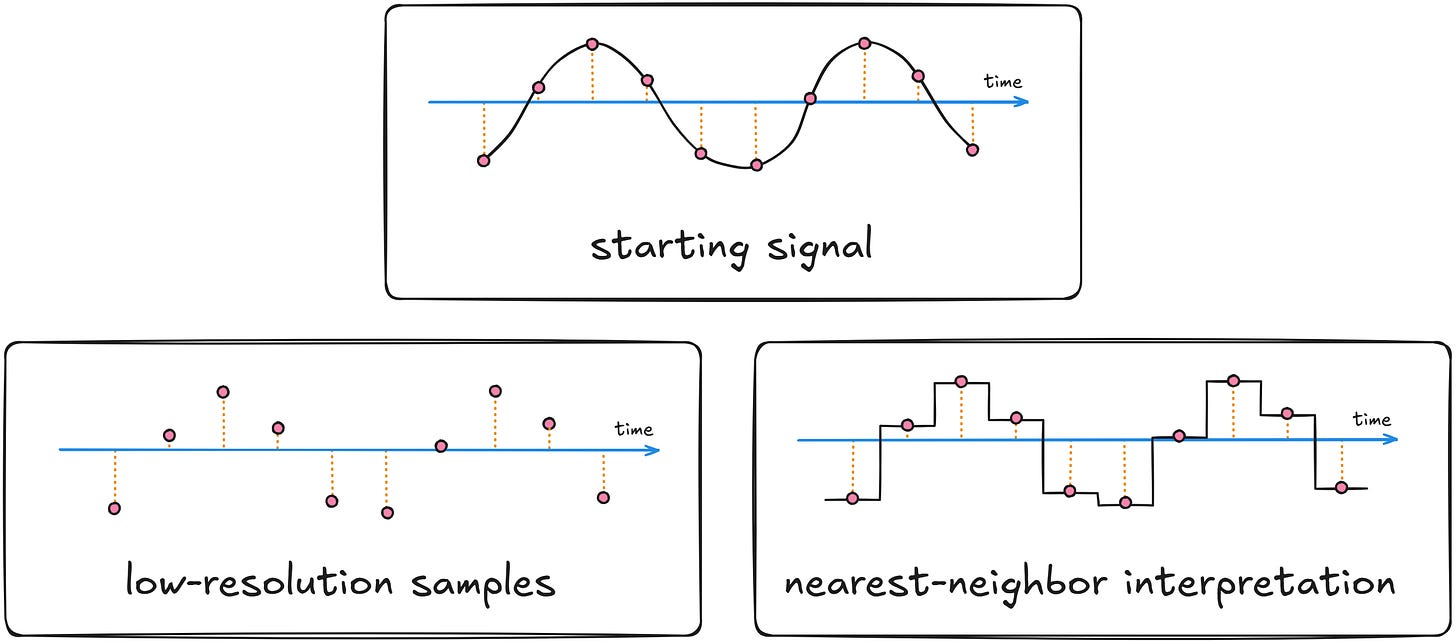
Our eyes do not pay attention to patterns on a computer screen, but the cochlea is a complex mechanical structure that does not measure sound pressure levels; Instead, it consists of groups of different nerve cells sensitive to different sine-wave frequencies. Sudden jumps in the waveform are treated as wideband noise that was not present in the original audio stream.

The problem is easy to solve: we can run the jagged wave through a rolling-average filter, which is equivalent to blurring a pixelated image to remove artifacts:

But this raises another question: would the effect be the same if we kept the original 44.1 kHz sampling rate but reduced the bit depth of each sample in the file?

/* Assumes signed int16_t buffer, produces n + 1 levels for even n. */

for (int i = 0; i < len; i++) {

  int div = 32767 / (levels / 2);
  buf[i] = round(((float)buf[i]) / div) * div;

}

The answer is yes and no: because the frequency of injected errors will be very high on average, we get whispers instead of screams:

Also note that loss of fidelity occurs much more rapidly for audio than for quantized images!

As for whispering, it is inherent in any attempt to play quantized audio; this is the reason digital-to-analog converters Your computer and audio gear usually needs to include some form of lowpass filtering. Your sound card has that, but we’ve injected more errors into the circuitry than those designed to hide.

But enough with image filters that ruin audio: we can also try some audio filters that ruin images! Let’s start by adding a slightly delayed and attenuated copy of the data stream to ourselves:

for (int i = shift; i < len; i++)
  buf[i] = (5 * buf[i] + 4 * buf[i - shift]) / 9;

Check it out:

For photographs, small offsets result in an unattractive blur, while larger offsets produce a strange “double exposure” look. For audio, the approach gives rise to a large and important family of filters. Small delays give the impression of a live performance in a small room; Large delays sound like echo in a large hall. Phase-shifted signals create effects like a “flangeer” or “phaser”, pitch-shifted echoes sound like a chorus, and so on.

So far, we have been working in the time domain, but we can also analyze data in the frequency domain; Any finite signal can be decomposed into a sum of sine waves with different amplitude, phase and frequency. The two most common conversion methods are discrete fourier transform and discrete cosine transform, but there are More quirky options to choose from If you are so inclined.

For images, the frequency-domain view is rarely used for editing because almost all transformations produce visual artifacts; The technique is used for compression, feature detection and noise removal, but no more; This can be used to sharpen or blur images, but there are easier ways to do it without FFT.

For audio, the story is different. For example, this approach makes it much easier to build vocoders that modulate the output from other devices to resemble human speech, or develop systems such as Auto-Tune, which make out-of-tune singing sounds sound passable.

In a previous article, I shared a simple implementation of Fast Fourier Transform (FFT) in C:

void __fft_int(complex* buf, complex* tmp, 
               const uint32_t len, const uint32_t step) {

  if (step >= len) return;
  __fft_int(tmp, buf, len, step * 2);
  __fft_int(tmp + step, buf + step, len, step * 2);

  for (uint32_t pos = 0; pos < len; pos += 2 * step) {
    complex t = cexp(-I * M_PI * pos / len) * tmp[pos + step];
    buf[pos / 2] = tmp[pos] + t;
    buf[(pos + len) / 2] = tmp[pos] - t;
  }

}

void in_place_fft(complex* buf, const uint32_t len) {
  complex tmp[len];
  memcpy(tmp, buf, sizeof(tmp));
  __fft_int(buf, tmp, len, 1);
} 

Unfortunately, the transformation gives us good output only when the input buffer contains approximately constant signals; The more variation in the analysis window, the more blurry and understandable the frequency-domain image will be. This means that we can’t take the entire song, run it through the C function above, and expect useful results.

Instead, we need to chop the track into smaller chunks, usually around 20-100 ms. This is long enough so that each slice can contain a reasonable number of samples, but short enough to more or less represent a transient “steady state” of the underlying waveform.

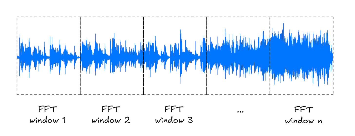
If we run the FFT function on each of these windows separately, each output will tell us about the frequencies distributed in that time slice; We can string these outputs together into a spectrogram, plotting how the frequencies (vertical axis) change over time (horizontal axis):

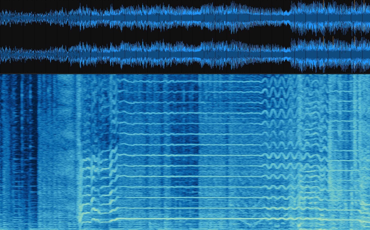
Alas, this method is not suited for audio editing: if we perform separate frequency-domain transformations in each window and then convert the data to time domain, there is no guarantee that the end of the reconstructed waveform for the window will match. n The front of the waveform will still align perfectly to the window. n + 1We are likely to end up with clicks and other audio artifacts where the FFT windows meet,

A clever solution to the problem is to use the Han function for windowing. In short, we multiply the waveform in each time slice by the value this , Sin²(Tea)Where? Tea Scaled so that each window starts at zero and ends at zero t = π. This results in a sinusoidal shape that has zero values ​​near the edges of the buffer and peaks at 1 in the middle:

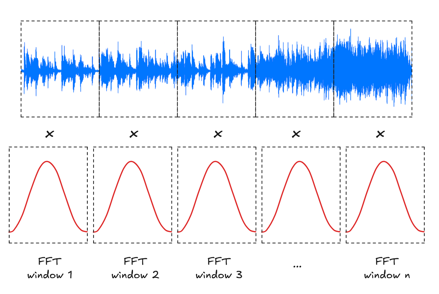
It is difficult to see how this would help: the result of the operation is that the input waveform is attenuated by a repeating sinusoidal pattern, and the same attenuation will carry over to the reconstructed waveform after the FFT.

The trick is to compute another sequence of “halfway” FFT windows of the same size that overlap the existing window (second row below):

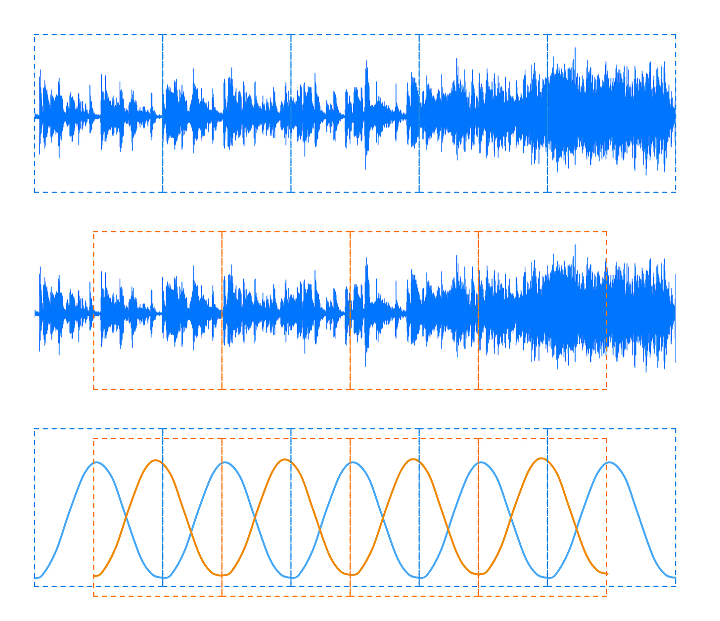
This leaves us with an output waveform that attenuates as the repetition Sin² pattern that begins at the beginning of the clip, and another wave form that is attenuated by a similar Sin² Half of the pattern cycle changed. The second pattern can also be written as ole²,

With this in mind, we can write the equation for reconstructed waves as:

<

div data-component-name=”Latex” class=”pencraft pc-display-flex pc-paddingTop-4px pc-paddingBottom-4px pc-justifyContent-center pc-reset flex-grow-rzmknG latex-rendered”>

(\begin{array}{c} out_1



<a href